At IPUMS we continuously enhance our data products with newly available datasets, adding new variables and improvements to existing variables. We do this with the “Data Conversion Program”, a C++ application built to transform census and survey data into “harmonized” micro-data. When you visit ipums.org and make data extracts, you’re downloading data developed with the DCP.
Developing additions to our data often necessitate repeatedly regenerating all datasets for data quality checks (regression testing: did we break anything) and checking on variables available across many datasets while they are a work in progress, up until a public release.
The DCP has been described as “ETL on steroids” (ETL == Extract, Transform, Load.) It reads in census or survey records, transforms and adds computed values on those records and writes them out to a common format. It applies both large amounts of simple transforms – which change as researchers work on perfecting the output they want – and more complex transforms and computations. If you’re familiar with machine learning, think of these computations as ML “features.” These typically draw on the more simple transforms as their inputs. Another way to think of the _DCP is as a specialized big data execution engine just for complex, structured social science micro-data.
The more frequently we can regenerate large groups of datasets the faster our researchers can get feedback on their changes. And as a bonus fewer compute resources are needed to do the same work, even if we don’t always need many iterations of a data production run. Throwing hardware at the data production has help speed up the process. However it was pretty clear for a while that there were opportunities to make the DCP itself significantly faster.
Recent refactoring and code deletion (always nice) gave me the chance to introduce experimental optimizations to the Data Conversion Program. Once in place, these improvements cut time required to produce an entire data product’s set of datasets to between one half and one fifth the original amount of time.
Around the same time as the optimizations we’re looking at were done, we also switched to default compression of all DCP output; the sheer volume of uncompressed data had become a bottleneck when running many parallel jobs on our storage infrastructure. Sizes of many datasets were growing quickly at this time. We also switched to default compression of inputs to DCP where possible. While I won’t go into this topic more in these posts, it should be clear that a crucial step to optimizing data intensive applications is to minimize the volumes of data going in and out.
There were three types of optimizations to the DCP application code:
- Replacing slow algorithms in user-supplied code, discovered through profiling
- Switching to a faster hash table implementation throughout the _DCP code
- Refactoring bottleneck code to use a more data-oriented approach
The first of these effected only certain datasets with large household sizes; it’s not really useful to compare optimization (1) with (2) or (3) to the baseline because of the bi-modal distribution of the improvements. For effected datasets the speed-up was ten to thirty times and for the rest it was negligible. [1]
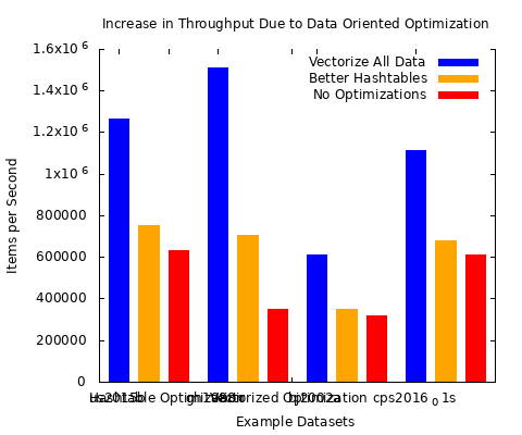
The second type – the hash table substitution – improved processing times on datasets everywhere with some products more than others; and the third – the data oriented refactoring – yielded the most improvement.
Results

Higher is better – more data per second.
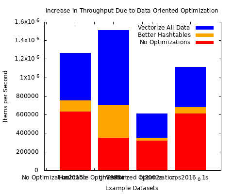
The red shows the baseline performance; the orange represents the amount of speed-up gained with the hash table substitution. The blue represents the additional speed-up of data-oriented refactoring of key bottleneck code.
Here’s a more compact form of the same data.

The following posts will go into detail about each of the optimizations, I cover the tools and approaches I used to achieve the big speed improvements shown here.
The take-away is that even when starting with a reasonably fast C++ application there may be lots of opportunities to dramatically improve performance. In the case of DCP we enabled throughput that otherwise would have required three to four times as many compute cluster nodes which aren’t cheap.
[1] Certain user-supplied algorithms were O(n^2) where n was the household size (number of people living in the household.) Certain households in the new datasets contained households with thousands of people instead of the previous maximum of sixty.For the majority of small sized households the differences in the algorithms before and after optimization was small similar to how a bubble sort on a small number of elements can be nearly or even faster than a merge sort or quick sort.